KQL Toolbox is officially live!

As part of this new KQL Toolbox series, I bring you practical, reusable KQL snippets straight from the trenches of real-world Microsoft Sentinel work. Think of it as your regular “KQL vitamin:” small dose, big impact. And today we’re kicking things off with the one question every SecOps team eventually asks: “Where is all my ingest money going?” 💸

Visualize and Price Your Billable Ingest Trends

If you’re running a SIEM or XDR platform and not looking at your ingest patterns regularly… you’re essentially flying blind on one of the biggest drivers of your security bill. This week’s KQL Toolbox article is all about shining the spotlight on your billable data ingestion in Microsoft Sentinel Log Analytics over the last 90 days—first visually, then in cold hard cash. 💰

Today, we’re going to look at three useful iterations of the same query:

Iteration 1 – “Show me billable GB per day, by solution, as a chart.”
Iteration 2 – “Roll it up per day, in GB and dollars.”
Iteration 3 – “Dress it up with STRCAT( )”

⚡Check out all 3 query iterations on my GitHub.

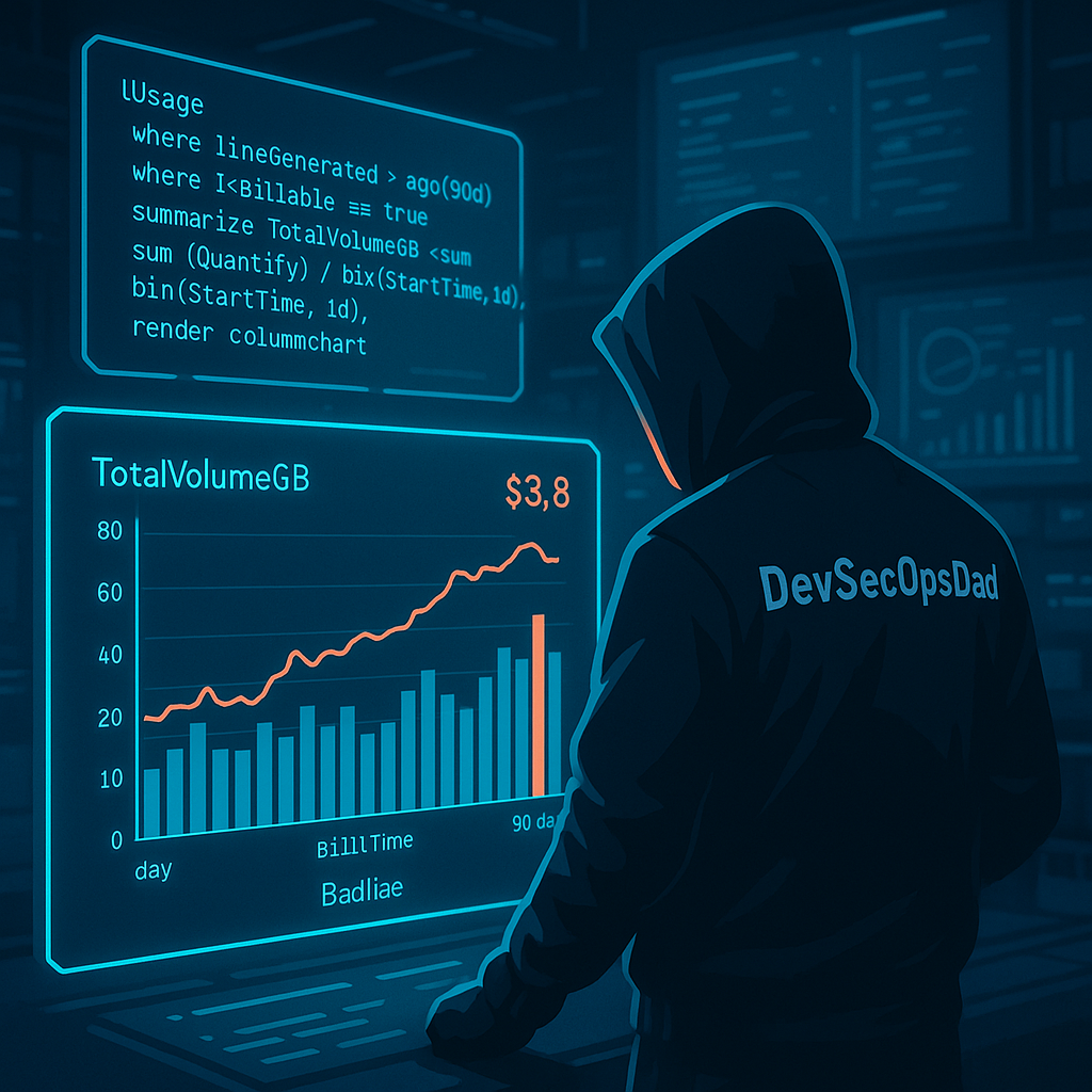
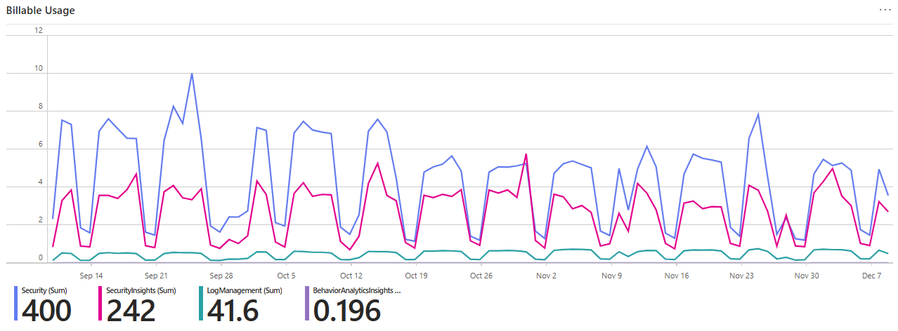
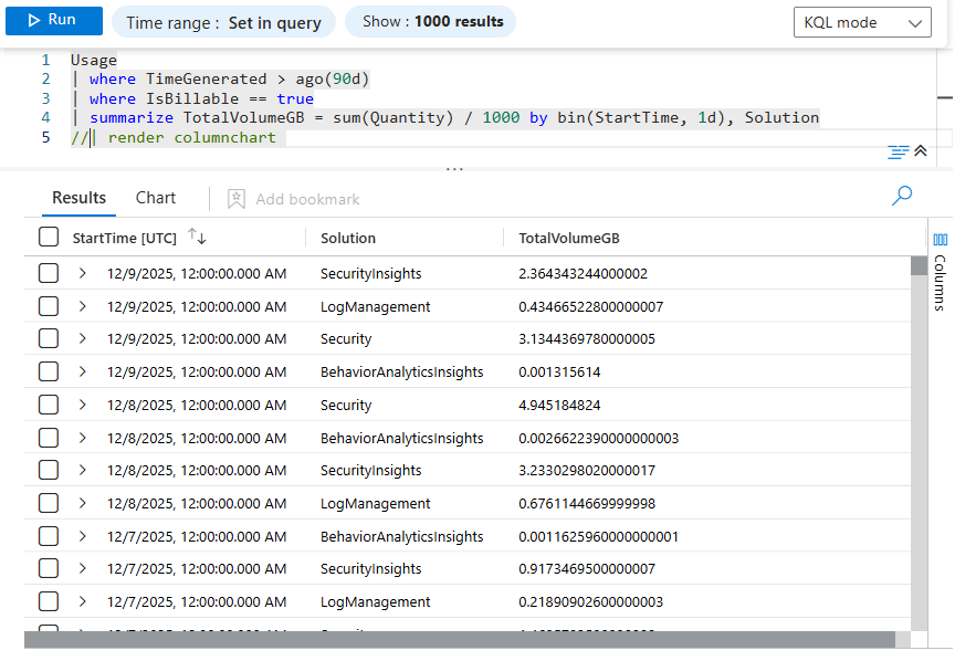
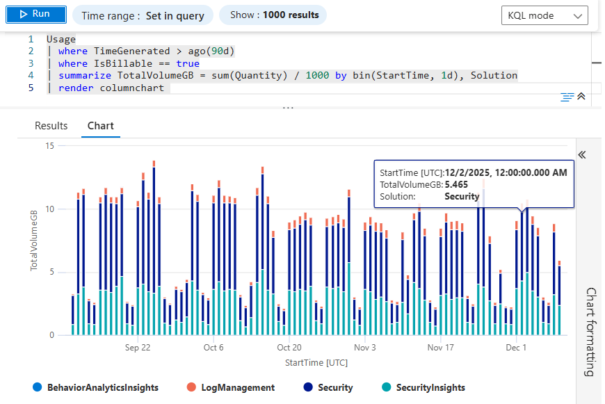
Query 1 – Billable GB per Day, by Solution (Column Chart)

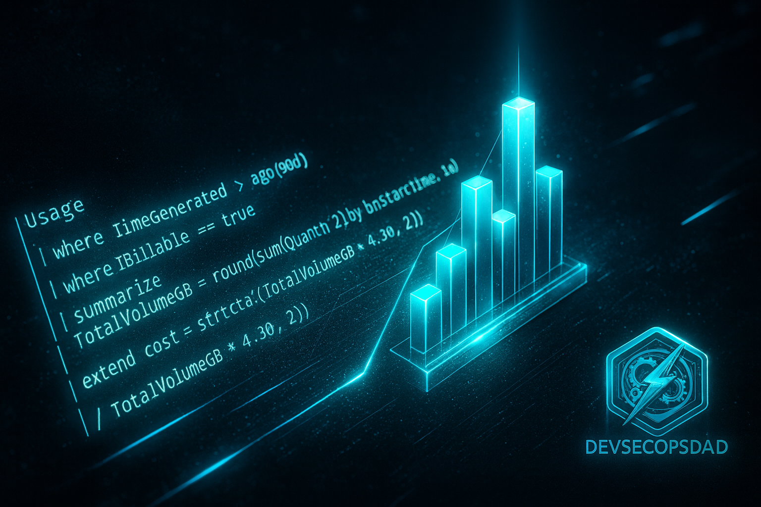
Usage
| where TimeGenerated > ago(90d)
| where IsBillable == true
| summarize TotalVolumeGB = sum(Quantity) / 1000 by bin(TimeGenerated, 1d), Solution
| render timechart

Line-by-line breakdown:

1.) `Usage`

This built-in table in Log Analytics acts as your ingest ledger, tracking how much data you ingest and which solution (Security, LogManagement, etc.) is responsible.

2.) `| where TimeGenerated > ago(90d)`

We’re scoping to the last 90 days of data. Great window for:

QBRs (Quarterly Business Reviews)
Trend analysis (did that new connector you added spike costs?)
Before/after reviews (e.g., “we tuned noisy logs here — did it work?”)

You can tweak 90d to anything you want: 30d, 7d, 365d, etc. Even 1h for an hour or 2m for two minutes.

💡 Pro-Tip:

Use 30d for Monthy reports; switch to 90 days at the end of the quarter to pivot to a quarterly report 😎

Use 5m to check if something you did affected ingest cost and immediately confirm whether you broke something 😅

3.) `| where IsBillable == true`

This is where the magic happens. We only care about records that count toward your bill. Some logs might be free or included (e.g., certain platform logs). IsBillable == true filters out the noise, leaving only data that actually costs you money.

4.) `| summarize TotalVolumeGB = sum(Quantity) / 1000 by bin(TimeGenerated, 1d), Solution`

This line does a lot of work:

sum(Quantity) – Each record has a Quantity field representing the size of data ingested (in MB).
/ 1000 – Convert MB to approximate GB (1000 MB ≈ 1 GB). This is a “marketing GB” vs “binary GB” thing; we’ll tighten this up in Query 2 and discuss how we got here later on.
TotalVolumeGB = ... – We give that result a friendly column name.
by bin(TimeGenerated, 1d), Solution – We group our data by:
- bin(TimeGenerated, 1d) – Buckets by day (based on TimeGenerated).
- Solution – Breaks the totals down per solution (e.g., Security, SecurityInsights, Microsoft Sentinel, etc.).

So you end up with:

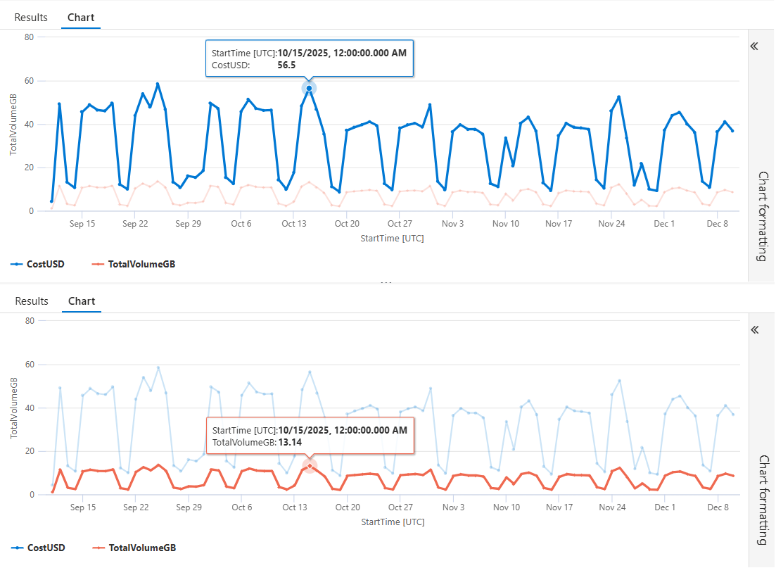
5.) `| render columnchart`

Finally, instead of returning a table, we render a visual:

X-axis: Date (per day)
Y-axis: GB ingested
Legend: Solution

This is the “Executive Slide” line. It gives you an instant sense of:

Which solutions are the main cost drivers.
Whether your ingest is stable, trending up, or spiking all over the place.
Where to focus tuning and data hygiene efforts.

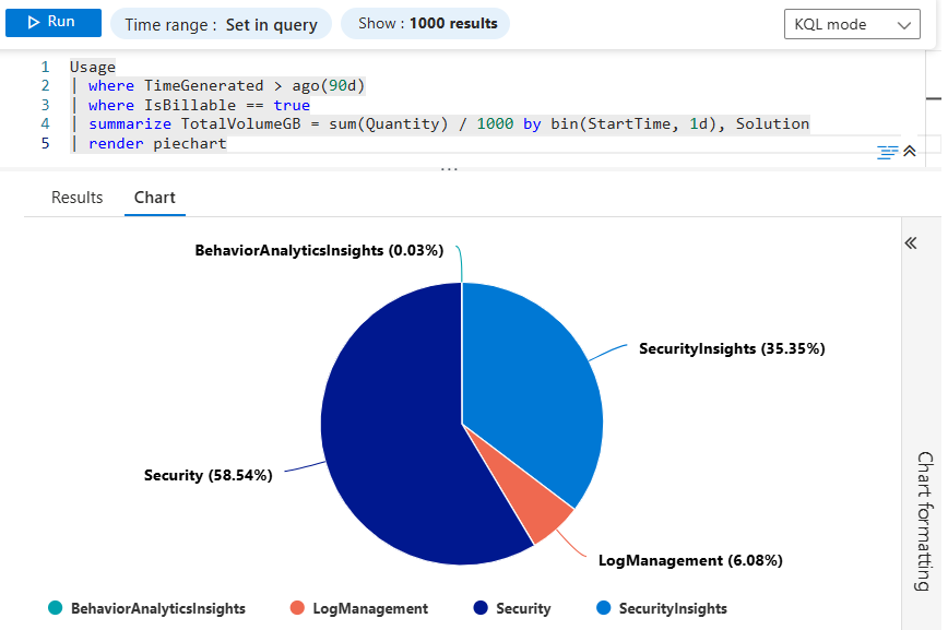
Don’t forget about pie charts too, for quickly identifying the heaviest drivers for ingest cost at a glance…

This is perfect for eyeballing trends and for screenshots in decks, QBRs, and “hey, what happened here?” emails.

Query 2 – Same Data, But Now With Actual Cost 🤑

⚡Check out all 3 query iterations on my GitHub.

Once you find a spike, the next question is always: “Okay, but how much is that in dollars?” 💵

Let’s look at the upgraded query:

Usage
| where TimeGenerated > ago(90d)
| where IsBillable == true
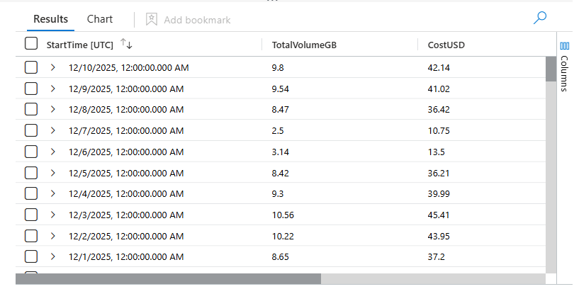
| summarize TotalVolumeGB = round(sum(Quantity) / 1024, 2) by bin(TimeGenerated, 1d)
| extend CostUSD = round(TotalVolumeGB * 4.30, 2)

What’s New Compared to Query 1?

Query 1 broke down billable ingest per Solution, which is perfect for “what’s noisy?” analysis. Query 2 shifts gears: it gives you total ingest per day, rolled up across the entire workspace, plus a dollar cost for each day.

Here’s what actually changed:

Solution was removed from summarize.
Instead of getting a bar per Solution per day, we now get one total per day.
This makes the output ideal for cost trending, budgeting, and forecasting.
Switched from / 1000 to / 1024, and added round().
Using 1024 MB = 1 GiB is more accurate for log volume math; Gigabyte vs. Gibibyte accuracy is discussed later
round(..., 2) keeps the numbers tidy and currency-friendly.
Added a cost column

This allows you to translate raw ingest volume into actual dollars, in-line with your workspace’s per-GB price. Let’s break down how this works in more detail, line-by-line…

1.) `summarize TotalVolumeGB = round(sum(Quantity) / 1024, 2) by bin(TimeGenerated, 1d)`

The front half of the query stays familiar: same Usage table, same 90-day window, same IsBillable == true.

But now the behavior changes a little:

sum(Quantity) – We still total all billable MB.
/ 1024 – Converts MB → GiB with binary precision.
round(..., 2) – Ensures readable values (e.g., 135.42, not 135.41893721).
And instead of grouping by Solution, we group only by the date (bin(TimeGenerated, 1d)), producing one record per calendar day. This gives you a clean daily total billable volume.

2.) `| extend CostUSD = round(TotalVolumeGB * 4.30, 2)`

Now we turn those GB into real money:

TotalVolumeGB * 4.30 – Multiplies by the per-GB price (e.g., $4.30/GB for East US on the Pay-As-You-Go commitment tier).
- 💲Swap 4.30 with your workspace’s actual price from Microsoft’s Sentinel pricing page.
round(..., 2) – Standard currency rounding to the second decimal place. Replace 2 with 3 to include three decimal places in your results, etc.

You now have a simple, finance-friendly daily ledger of your Sentinel costs — perfect for:

CSV/Excel exports
Monthly reporting
QBR deck visuals
Cost justification (filter noisy logs, reduce retention, move data to cheaper tiers)

📊 And if you want the classic visualization, just tack this on the end: | render columnchart

Dress it up with `STRCAT()!` 😎

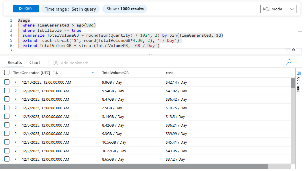
strcat() in KQL concatenates multiple values into a single string. In this case, we’re taking a number, a currency symbol, and a suffix, and merging them into one formatted display value, transforming numeric columns into string-formatted display values. That’s key for converting data that had mathematical meaning into purely presentation-friendly text.. Let’s break it down…

1. Formatting Daily Cost:

| extend cost = strcat('$', round(TotalVolumeGB * 4.30, 2), ' / Day')

What this line does:

Takes TotalVolumeGB (a number)
Multiplies it by your per-GB cost rate (4.30)
Rounds the result to 2 decimal places
Converts the numeric cost into a string
Prepends a $
Appends ” / Day”

So: 52.80 becomes $52.80 / Day

2. Converting TotalVolumeGB to a Display-Ready String

| extend TotalVolumeGB = strcat(TotalVolumeGB, 'GB / Day')

What this line does

Takes your numeric TotalVolumeGB
Appends the string ‘GB / Day’
Converts the entire result into a string

So: 12.54 becomes 12.54GB / Day

3. 🤔 Why?

Because you’re shifting the output from analysis-ready to human-ready. Once the numbers are formatted, they’re much easier to interpret in:

Workbooks & dashboards
Exports and email reports
SOC/Jupyter visuals
Blog posts 👋😁
Client-facing deliverables

In other words, you’re preparing the data for presentation, not additional math — a common pattern whenever the final output needs to be clean, readable, and report-ready.

4. ⚠️ Pitfall to Watch Out for

Here’s the nuance when using strcat()… After this line, cost is no longer numeric… Meaning You can no longer:

sum cost

average cost

chart cost as a numeric measure

convert GB → MB

re-round values

bucket by numeric thresholds

feed into a chart that expects a number

👉 This column effectively becomes display-only 👀

🧠 Deeper Discussion: Why Format at the End?

This pattern is excellent as long as you’re done calculating because once a column becomes a string → it stops being useful for math. If you ever need raw values again, formatting early could shoot you in the foot.

💡Best practice tip: If you need raw numeric values and formatted output, created new, separate, “formatted” columns with something like this:

| extend TotalVolumeGB_Formatted = strcat(TotalVolumeGB, 'GB / Day')

| extend cost_Formatted = strcat('$', round(TotalVolumeGB * 4.30, 2), ' / Day')

This keeps:

TotalVolumeGB as float
Cost as float
formatted versions as strings
things looking slick 😎

🛠️ Run these query now and compare the last 30, 60, and 90 days. If you see unexpected spikes, you’ve already found optimization opportunities. Don’t wait until Azure billing surprises you — measure it before it measures you.

📝 Quick Note: Gibibytes vs Gigabytes

You’ll sometimes see data measured in gigabytes (GB) and other times in gibibytes (GiB) — and while they sound similar, they’re not the same.

Gigabytes (GB) use base-10 math, the same system your hard drive or cloud provider marketing uses: 1 GB = 1,000,000,000 bytes
Gibibytes (GiB) use base-2 math, which matches how computers actually store and address memory: 1 GiB = 1,073,741,824 bytes (1024³)

In other words, 1 GiB is about 7% larger than 1 GB. So depending on whether a platform reports usage in GB or GiB, the numbers may look slightly different even though the underlying data is identical. This matters in KQL because some tables report usage in binary units (GiB) while pricing calculators often use decimal units (GB). The important part isn’t which one you choose — it’s that you apply it consistently when analyzing ingest trends or estimating cost.

💽 How We Ended Up With Gigabytes Instead of Gibibytes

For decades, the tech industry used the word gigabyte (GB) to describe both decimal and binary measurements — even though they’re not the same. This wasn’t intentional deception; it was simply convenient shorthand during the early personal computing era.

Hard drive manufacturers used decimal gigabytes (powers of 10) because it made capacity numbers round, clean, and easier to market.

1 GB = 1,000,000,000 bytes

Operating systems used binary measurements (powers of 2) because that’s how memory addressing actually works.

1 GiB = 1,073,741,824 bytes

For years, both groups called their units GB — which caused confusion as storage capacities grew. To fix the ambiguity, the International Electrotechnical Commission (IEC) introduced new binary-prefixed terms in 1998:

Kibibyte (KiB)
Mebibyte (MiB)
Gibibyte (GiB)

…and so on

The idea was simple: Use GB for decimal, GiB for binary. But adoption was slow: Developers and OS vendors (Linux, BSD, macOS) gradually embraced the binary IEC terms. Windows kept using “GB” for binary values for many years. Cloud platforms went mixed — pricing calculators tended to use GB (decimal), but logs and metrics often used binary math. By the time cloud computing exploded, GB had already become the de facto public-facing unit, while GiB remained the technically correct measurement under the hood.

Today, both exist because both are useful:

GB → pricing, marketing, cloud billing
GiB → memory, file systems, compute workloads, low-level metrics

And because the names sound similar, the confusion never totally went away — which is why it’s worth calling out in a KQL series where cost math actually matters.

↔️ Quick Comparison

Unit	Bytes	Notes
1 GB	1,000,000,000 bytes	Decimal (SI) — what vendors use
1 GiB	1,073,741,824 bytes	Binary (IEC) — what Log Analytics / Microsoft usage uses internally

⏰ Bonus Discussion: StartTime vs TimeGenerated

Some of my sharper readers may have noticed that a few screenshots used StartTime instead of TimeGenerated. That one’s on me (#DevSecOops 😅); Just like my GB vs GiB rant, I occasionally commit crimes against precision — so here’s a clear breakdown of what these two fields actually represent, and why it matters for cost analysis.

TimeGenerated

This is the actual timestamp when the Usage record was logged.
Every row in Log Analytics has this column.
In the Usage table, it represents when the usage event was recorded.

StartTime

This column exists specifically in the Usage table.
It represents the start of the billing interval for that usage event.
It often aligns with internal computation windows used by Microsoft for calculating ingest cost, retention, or other metered operations.

In other words:

TimeGenerated = When the record was written.
StartTime = When the billable usage window began.

🤓 Which one should you use for daily cost charts?

The Usage table’s StartTime is not guaranteed to align perfectly with the calendar day boundary.

It may reflect:

the start of a metering window
ingestion pipeline processing
hourly or sub-daily aggregation cycles inside the Microsoft billing engine

That means:

Days may start at strange hours (e.g., 01:00 UTC or 17:00 UTC)
Some bins may appear empty or shifted
Visuals may look offset or inconsistent

🎯 For clean, calendar-based daily trends, use TimeGenerated with bin(1d), like this: StartTime = bin(TimeGenerated, 1d)

This gives you:

Exactly one bucket per calendar day
Continuous, predictable daily bins
No risk of odd Usage-table billing boundaries messing with grouping

📚 Want to go deeper?

From logs and scripts to judgment and evidence — the DevSecOpsDad Toolbox shows how to operate Microsoft security platforms defensibly, not just effectively.

🛠️ KQL Toolbox: Turning Logs into Decisions in Microsoft Sentinel

🧰 PowerShell Toolbox: Hands-On Automation for Auditing and Defense

📖 Ultimate Microsoft XDR for Full Spectrum Cyber Defense
Real-world detections, Sentinel, Defender XDR, and Entra ID — end to end.

🔗 References (good to keep handy)

Other Fun Stuff…

DevSecOpsDad.com

KQL Toolbox is officially live!

Visualize and Price Your Billable Ingest Trends

⚡Check out all 3 query iterations on my GitHub.

Query 1 – Billable GB per Day, by Solution (Column Chart)

Line-by-line breakdown:

1.) Usage

2.) | where TimeGenerated > ago(90d)

3.) | where IsBillable == true

4.) | summarize TotalVolumeGB = sum(Quantity) / 1000 by bin(TimeGenerated, 1d), Solution

5.) | render columnchart

Query 2 – Same Data, But Now With Actual Cost 🤑

⚡Check out all 3 query iterations on my GitHub.

What’s New Compared to Query 1?

1.) summarize TotalVolumeGB = round(sum(Quantity) / 1024, 2) by bin(TimeGenerated, 1d)

2.) | extend CostUSD = round(TotalVolumeGB * 4.30, 2)

Dress it up with STRCAT()! 😎

1. Formatting Daily Cost:

2. Converting TotalVolumeGB to a Display-Ready String

3. 🤔 Why?

4. ⚠️ Pitfall to Watch Out for

🧠 Deeper Discussion: Why Format at the End?

📝 Quick Note: Gibibytes vs Gigabytes

💽 How We Ended Up With Gigabytes Instead of Gibibytes

↔️ Quick Comparison

⏰ Bonus Discussion: StartTime vs TimeGenerated

🤓 Which one should you use for daily cost charts?

📚 Want to go deeper?

🔗 References (good to keep handy)

Other Fun Stuff…

1.) `Usage`

2.) `| where TimeGenerated > ago(90d)`

3.) `| where IsBillable == true`

4.) `| summarize TotalVolumeGB = sum(Quantity) / 1000 by bin(TimeGenerated, 1d), Solution`

5.) `| render columnchart`

1.) `summarize TotalVolumeGB = round(sum(Quantity) / 1024, 2) by bin(TimeGenerated, 1d)`

2.) `| extend CostUSD = round(TotalVolumeGB * 4.30, 2)`

Dress it up with `STRCAT()!` 😎