KQL Toolbox #4: What Changed? Finding Log Sources with the Biggest Delta in Volume & Cost

Welcome back to KQL Toolbox 👋

In KQL Toolbox #1, we learned how to measure Microsoft Sentinel ingest and translate it into real dollars. In KQL Toolbox #2, we identified which data sources were driving that cost. And in KQL Toolbox #3, we drilled all the way down to specific Event IDs, accounts, and devices generating noise.

So at this point? You can already answer:

What’s expensive
What’s noisy
Who’s responsible

But once you’ve got those basics down, there’s one question every SOC analyst, engineer, and cost owner eventually asks: “Okay… what changed?”

Because in the real world, cost spikes and alert storms rarely come from what’s always been there — they come from sudden shifts, like:

A misconfigured data connector
A new audit policy rolled out too broadly
A broken agent stuck in a logging loop
Or a “temporary” change that quietly became permanent

That’s where this week’s KQL comes in; Instead of ranking data sources by total volume or total cost, KQL Toolbox #4 focuses on delta — identifying which log sources have experienced the largest change in billable volume compared to a historical baseline.

And the best part?

This allows you to stop guessing, stop doom-scrolling charts, and immediately zero in on what deserves investigation first.

If you’re working in Azure Monitor Logs / Log Analytics or Microsoft Sentinel, tracking down why billable volume is changing is one of the most common (and most expensive) operational headaches. Whether it’s a cloud migration, a new app rollout, a misconfigured agent, or just normal growth — understanding what’s driving the delta is critical for budgeting, troubleshooting, and overall SOC hygiene.

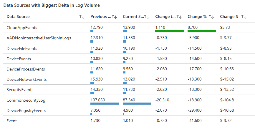
Today we’re going to unpack one of my favorite preventive analytics queries: “Data Sources with Biggest Delta in Log Volume.” 💸

Let’s break it down, put it to work, then crank it up a notch — ‘cause this is DevSecOpsDad. 😎

🕵️ What this query is trying to answer

“Which data sources changed the most in billable log volume when comparing the last 30 days vs the 30 days before that?”

It does this by:

defining two time windows
summarizing billable Usage by DataType
doing a full outer join so new/discontinued sources still show up
calculating absolute delta (GB) and percent delta (%)
returning the top 5 biggest absolute swings

//This query:
//-->Finds the exact time ranges for comparison periods (previous 30 days vs current 30 days)
//-->Calculates total GB for each data source in both periods
//-->Joins the results to show the comparison
//-->Calculates both absolute and percentage changes
//-->Shows top 5 sources with biggest absolute changes
//-->Handles cases where sources might be new or discontinued

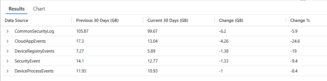
//The results include:
//-->Data Source name
//-->Volume for previous 30 days in GB
//-->Volume for current 30 days in GB
//-->Absolute change in GB
//-->Percentage change

// Capture the exact end of the "current" period by finding the latest
// billable Usage record in the workspace
let CurrentPeriod = toscalar(
    Usage                              // Query the Usage (billing) table
    | where IsBillable == true         // Only include billable ingestion
    | summarize max(TimeGenerated)     // Find the most recent billable record timestamp
);
// Define the start of the current 30-day comparison window
let CurrentStart = CurrentPeriod - 30d;   // Current window = last 30 days of data
// Define the start of the prior 30-day window
let PriorStart   = CurrentPeriod - 60d;   // Prior window starts 60 days before CurrentPeriod
// Define the end of the prior window so the two windows are perfectly adjacent
let PriorEnd     = CurrentStart;           // Prior window ends exactly where current begins
// Summarize total billable volume (GB) per data source for the prior period
let PriorData =
    Usage
    | where IsBillable == true                                 // Only billable ingestion
    | where TimeGenerated between (PriorStart .. PriorEnd)    // Filter to prior 30-day window
    | summarize PriorGB = round(todouble(sum(Quantity)) / 1024, 2)
        by DataType;                                          // Aggregate by data source (table)
// Summarize total billable volume (GB) per data source for the current period
let CurrentData =
    Usage
    | where IsBillable == true                                 // Only billable ingestion
    | where TimeGenerated between (CurrentStart .. CurrentPeriod) // Filter to current 30-day window
    | summarize CurrentGB = round(todouble(sum(Quantity)) / 1024, 2)
        by DataType;                                          // Aggregate by data source (table)
// Join prior and current datasets so we can compare changes
PriorData
| join kind=fullouter CurrentData on DataType                 // Include new and discontinued sources
| extend
    DataType  = coalesce(DataType, DataType1),                // Normalize DataType name after join
    PriorGB   = coalesce(PriorGB, 0.0),                        // Treat missing prior data as 0 GB
    CurrentGB = coalesce(CurrentGB, 0.0)                       // Treat missing current data as 0 GB
| project
    ['Data Source']            = DataType,                    // Friendly column name
    ['Previous 30 Days (GB)']  = PriorGB,                     // Prior period volume
    ['Current 30 Days (GB)']   = CurrentGB,                   // Current period volume
    ['Change (GB)']            = round(CurrentGB - PriorGB, 2), // Absolute volume change
    ['Change %']               =
        iif(
            PriorGB > 0,
            round(((CurrentGB - PriorGB) / PriorGB) * 100, 1), // Percent change when baseline exists
            100.0                                              // Fallback for brand-new sources
        )
| where
    ['Current 30 Days (GB)'] > 0
    or ['Previous 30 Days (GB)'] > 0                           // Remove rows with no activity at all
| top 5 by abs(['Change (GB)']) desc                           // Show the biggest movers (up or down)

👉 Grab the Copy-Paste ready KQL from my Github library here: 🔗 Log_Sources_with_Greatest_Delta.kql

🔍 Line-by-line breakdown

1️⃣ Establish the anchor point for time comparisons

let CurrentPeriod = toscalar(
    Usage
    | where IsBillable == true
    | summarize max(TimeGenerated)
);

What this does: Finds the latest billable ingestion timestamp in your workspace and stores it as a scalar value.

Why it matters: This becomes the true end boundary for your analysis — not “now,” but the most recent data you actually have. This prevents partial-day skew and ingestion delays from distorting comparisons.

2️⃣ Define perfectly symmetric time windows

let CurrentStart = CurrentPeriod - 30d;
let PriorStart   = CurrentPeriod - 60d;
let PriorEnd     = CurrentStart;

What this does –> Creates two back-to-back 30-day windows:

Prior: CurrentPeriod - 60d → CurrentPeriod - 30d
Current: CurrentPeriod - 30d → CurrentPeriod

Why it matters: This is true apples-to-apples comparison. Each window:

Is the same length
Touches the same “data freshness”
Has no overlap and no gaps

3️⃣ Calculate prior-period volume by data source

let PriorData =
    Usage
    | where IsBillable == true
    | where TimeGenerated between (PriorStart .. PriorEnd)
    | summarize PriorGB = round(todouble(sum(Quantity)) / 1024, 2) by DataType;

What this does –> For each DataType (log table):

Sums billable ingestion (Quantity)
Converts MB → GB (GiB-ish)
Produces total volume for the prior 30-day window

Why it matters: This is your baseline behavior — what “normal” looked like.

4️⃣ Calculate current-period volume by data source

let CurrentData =
    Usage
    | where IsBillable == true
    | where TimeGenerated between (CurrentStart .. CurrentPeriod)
    | summarize CurrentGB = round(todouble(sum(Quantity)) / 1024, 2) by DataType;

What this does: Same aggregation as above, but for the current 30-day window.

Why it matters: Now you have two comparable datasets that describe how each log source behaved before and after.

5️⃣ Join prior and current data together

PriorData
| join kind=fullouter CurrentData on DataType

What this does: A fullouter join ensures you capture:

Data sources that existed before but disappeared
Data sources that are brand new
Data sources present in both periods

Why it matters: Delta analysis is useless if new or dropped sources vanish from the results.

6️⃣ Normalize nulls after the join

| extend
    DataType  = coalesce(DataType, DataType1),
    PriorGB   = coalesce(PriorGB, 0.0),
    CurrentGB = coalesce(CurrentGB, 0.0)

What this does:

Merges the two DataType columns created by the join
Converts missing values into zeros

Why it matters –> This makes math predictable:

New source → PriorGB = 0
Discontinued source → CurrentGB = 0

7️⃣ Calculate deltas and format output

| project
    ['Data Source']            = DataType,
    ['Previous 30 Days (GB)']  = PriorGB,
    ['Current 30 Days (GB)']   = CurrentGB,
    ['Change (GB)']            = round(CurrentGB - PriorGB, 2),
    ['Change %']               = iif(PriorGB > 0, round(((CurrentGB - PriorGB) / PriorGB) * 100, 1), 100.0)

What this does:

Computes absolute change in GB
Computes percentage change
Uses friendly column names for dashboards and screenshots

⚠️ Important nuance: When PriorGB == 0, percentage change is forced to 100.0 to avoid divide-by-zero — this really means “new data source”, not “exactly doubled.”

8️⃣ Remove meaningless rows

| where ['Current 30 Days (GB)'] > 0 or ['Previous 30 Days (GB)'] > 0

What this does: Filters out rows where nothing existed in either window.

9️⃣ Surface the biggest changes first

| top 5 by abs(['Change (GB)']) desc

What this does –> Ranks data sources by magnitude of change, regardless of direction:

Big increases
Big decreases

Why it matters –> Both are operational signals:

Increases → new noise or misconfiguration
Decreases → tuning success or broken ingestion

✅ Summary:

This query is essentially a “delta radar”:

prior 30 days vs current 30 days
per data source (DataType)
shows biggest swings first
includes new/discontinued sources via fullouter

⚔️ Steps to Operationalize

Run this query weekly (ops hygiene) and monthly (cost governance / QBR prep).
Pin results to a workbook tile called “Top DataType Movers (GB)”.
Establish an action loop:
- Identify the top mover(s)
- Pivot into that table (KQL Toolbox #2)
- Drill down to Event IDs / accounts / devices if applicable (KQL Toolbox #3)
- Document the cause + remediation in a lightweight change log

💡 Best practice: keep a “known expected deltas” list (month-end patching, migrations, major rollouts) so analysts don’t re-investigate planned change.

🛡️ Framework Mapping

NIST CSF DE.CM-1 / DE.CM-7 — Continuous monitoring detects abnormal changes in telemetry patterns.
NIST CSF DE.AE-1 — Supports baselining (“what normal looks like”) to detect deviation.
NIST CSF ID.RA-1 — Helps identify and prioritize sources of operational risk (misconfig / ingestion gaps).
CIS Control 8.2 / 8.5 — Audit log review + tuning to reduce noise and improve detection effectiveness.

“Okay… But How Much Did those GB’s just Cost?” 💰

Now that we’ve walked through a query that shows you which log sources have shifted the most in volume over the past 30-day window versus the 30 days before that (giving you eyes on where the activity moved), it’s time to bring financial context into the picture. Volume deltas alone are great for troubleshooting and operational insight, but when you’re preparing dashboards, reports, or QBR slides, your stakeholders care about dollars as much as gigabytes.

In the next query, we take the same comparison pattern — adjacent 30-day windows, full outer joins to capture new/discontinued sources, and ranking by magnitude of change — and enhance it with estimated cost impact based on your regional Sentinel ingest price. This lets you not only see what changed, but also what that change likely did to your bill, turning operational insight into business-relevant guidance you can act on and communicate effectively.

// -------------------------------
// Configuration / Tunables
// -------------------------------
let CostPerGB = 4.30;                      // <-- Sentinel ingest cost per GB (update per region)

let CurrentEnd = now();                    // <-- End of current window (query execution time)
let CurrentStart = CurrentEnd - 30d;       // <-- Start of current 30-day window
let PriorStart = CurrentEnd - 60d;         // <-- Start of prior 30-day window
let PriorEnd = CurrentStart;               // <-- End of prior window (exactly where current begins)


// -------------------------------
// Prior 30-Day Usage (Days -60 → -30)
// -------------------------------
let PriorData =
    Usage                                   // <-- Query the Usage (billing) table
    | where IsBillable == true              // <-- Only include billable ingestion
    | where TimeGenerated >= PriorStart     // <-- Prior window start (inclusive)
          and TimeGenerated < PriorEnd      // <-- Prior window end (exclusive, avoids overlap)
    | summarize                             // <-- Aggregate total ingest for that window
        PriorGB = round(
            todouble(sum(Quantity)) / 1024, // <-- Sum MB and convert to GB (MB → GB)
            2                               // <-- Round to 2 decimals
        )
        by DataType;                        // <-- Group by table / data source name


// -------------------------------
// Current 30-Day Usage (Days -30 → Now)
// -------------------------------
let CurrentData =
    Usage                                   // <-- Query the Usage (billing) table
    | where IsBillable == true              // <-- Only include billable ingestion
    | where TimeGenerated >= CurrentStart   // <-- Current window start (inclusive)
          and TimeGenerated <= CurrentEnd   // <-- Current window end (inclusive)
    | summarize                             // <-- Aggregate total ingest for that window
        CurrentGB = round(
            todouble(sum(Quantity)) / 1024, // <-- Sum MB and convert to GB (MB → GB)
            2                               // <-- Round to 2 decimals
        )
        by DataType;                        // <-- Group by table / data source name


// -------------------------------
// Comparison & Delta Analysis
// -------------------------------
PriorData
| join kind=fullouter                       // <-- Keep all sources (new/discontinued included)
    CurrentData
    on DataType                             // <-- Join on data source name
| extend
    PriorGB   = coalesce(PriorGB, 0.0),     // <-- Missing prior data becomes 0
    CurrentGB = coalesce(CurrentGB, 0.0),   // <-- Missing current data becomes 0
    ChangeGB  = CurrentGB - PriorGB         // <-- Compute raw GB delta (positive or negative)
| project
    ['Data Source']           = DataType,   // <-- Friendly output name
    ['Previous 30 Days (GB)'] = PriorGB,    // <-- Prior window volume
    ['Current 30 Days (GB)']  = CurrentGB,  // <-- Current window volume
    ['Change (GB)']           = round(      // <-- Rounded delta for display
        ChangeGB,
        2
    ),
    ['Change %'] =
        iif(
            PriorGB > 0,                    // <-- Only compute % change if baseline exists
            round(
                (ChangeGB / PriorGB) * 100, // <-- Percent change formula
                1
            ),
            real(null)                      // <-- If prior was 0, % is undefined (don’t fake it)
        ),
    ['Change $'] =
        strcat(
            '$',
            round(
                ChangeGB * CostPerGB,       // <-- Convert GB delta into estimated cost delta
                2
            )
        )
| where                                    // <-- Remove rows where both windows are 0
    ['Current 30 Days (GB)'] > 0
    or ['Previous 30 Days (GB)'] > 0
| top 10                                   // <-- Focus on the biggest movers
    by abs(['Change (GB)']) desc            // <-- Rank by magnitude (spike OR drop)

👉 Grab the Copy-Paste ready KQL from my Github library here: 🔗 Data Sources with Biggest Delta in Log Volume.kql

🔍 Line-by-line breakdown

1️⃣ Configuration / Tunables

let CostPerGB = 4.30; –> What it does: sets your Sentinel ingest price per GB (example value). Why it matters: lets you translate volume change into a $ delta, which is what gets attention in QBRs.

let CurrentEnd = now(); –> What it does: uses the current clock time as the end of your reporting window. Why it matters: this makes the query run “as of right now.”

let CurrentStart = CurrentEnd - 30d;
let PriorStart = CurrentEnd - 60d;
let PriorEnd = CurrentStart;

What it does: creates two adjacent 30-day windows:

Prior: -60d → -30d
Current: -30d → now

Why it matters: symmetry. Same duration, back-to-back, no gaps.

2️⃣ Prior 30-Day Usage

let PriorData =
    Usage
    | where IsBillable == true
    | where TimeGenerated >= PriorStart
          and TimeGenerated < PriorEnd
    | summarize PriorGB = round(todouble(sum(Quantity)) / 1024, 2) by DataType;

What this does for the prior window:

pulls billable Usage rows
filters to PriorStart through PriorEnd
sums Quantity by DataType
converts to GB and rounds

Why the end is exclusive (< PriorEnd): This is a subtle pro move. It prevents overlap with the current period boundary so the windows don’t double-count rows that land exactly on PriorEnd.

3️⃣ Current 30-Day Usage

let CurrentData =
    Usage
    | where IsBillable == true
    | where TimeGenerated >= CurrentStart
          and TimeGenerated <= CurrentEnd
    | summarize CurrentGB = round(todouble(sum(Quantity)) / 1024, 2) by DataType;

What this does: Same aggregation, but for the current window.

4️⃣ Join + Delta Analysis

Join:

PriorData
| join kind=fullouter CurrentData on DataType

What it does: combines both datasets and keeps everything from both sides.

Why it matters –> this ensures you still see:

brand new data sources (only in current)
discontinued sources (only in prior)

Extend:

| extend
    PriorGB   = coalesce(PriorGB, 0.0),
    CurrentGB = coalesce(CurrentGB, 0.0),
    ChangeGB  = CurrentGB - PriorGB

What it does: null prior/current volumes become 0. ChangeGB becomes your clean delta value.
Why it matters: you can now do math safely without null checks everywhere.

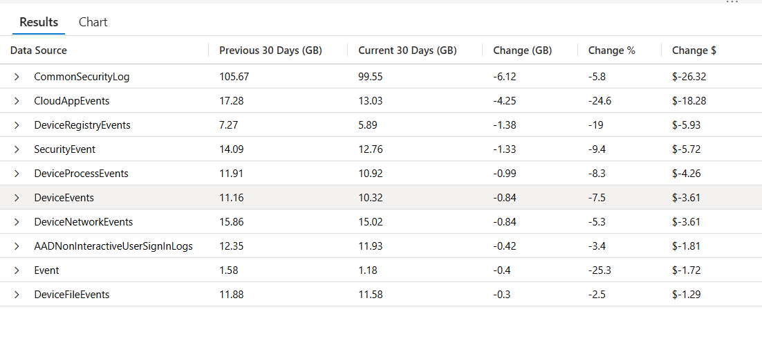
5️⃣ Output shaping: GB, %, and $ (project)

GB 👇

| project
    ['Data Source']           = DataType,
    ['Previous 30 Days (GB)'] = PriorGB,
    ['Current 30 Days (GB)']  = CurrentGB,
    ['Change (GB)']           = round(ChangeGB, 2),

What it does: makes the results human-friendly (perfect for blog screenshots and workbooks).

% 👇

['Change %'] =
    iif(
        PriorGB > 0,
        round((ChangeGB / PriorGB) * 100, 1),
        real(null)
    ),

What it does: only calculates percent change when a baseline exists.
Why it matters: this is a quality upgrade over the earlier approach that forced “100%” for new sources.

Here, new sources show null (more honest), which signals “this source is NEW.”

💲👇

['Change $'] =
    strcat(
        '$',
        round(ChangeGB * CostPerGB, 2)
    )

What it does: converts the GB delta into an estimated cost delta.
Why it matters: your top-10 list is no longer just “volume changed.”
It becomes “volume changed and here’s what it likely did to the bill.”

6️⃣ Clean-up and ranking

| where ['Current 30 Days (GB)'] > 0 or ['Previous 30 Days (GB)'] > 0`

What it does: removes rows with no activity at all.

| top 10 by abs(['Change (GB)']) desc

What it does: returns the biggest movers by magnitude, whether spike or drop.
Why it matters –> both directions are signals:
- Spike: new noise, misconfig, or growth
- Drop: tuning success… or broken ingestion

This looks slick as a part of a cost optimization workbook…

⚔️ Steps to Operationalize

Run monthly as part of a Cost/Value review (and pre-QBR).

Store results in a workbook section titled “Delta Impact ($)”.

Operationalize stakeholder comms:
- Security / SOC gets the “what changed and why” story
- Finance / leadership gets “what changed and what it cost” story

Use the output to drive targeted actions:
- tune connector settings
- transformation rules (where supported)
- move low-value telemetry to cheaper tiers / alternative storage patterns
- retention adjustments (carefully)

🛡️ Framework Mapping

NIST CSF ID.GV-1 / ID.GV-3 — Governance + risk management decisions informed by measurable telemetry impact.
NIST CSF PR.IP-1 — Supports configuration management processes (logging configs are “config”).
NIST CSF DE.CM-7 — Monitoring includes cost-relevant telemetry changes impacting detection operations.
CIS Control 17.3 (Service Provider / Cloud Mgmt) + CIS 8 — Managing cloud telemetry and audit logs as operational controls (especially in Sentinel/Log Analytics).

📋 Next Steps:

Now that you can quickly identify which log sources changed the most — and what that change likely cost, here are a few practical ways to put this query to work:

Drill down on the offenders
- Take the top data source(s) from this output and pivot back into your earlier toolbox queries:
Use KQL Toolbox #2 to break the table down further by volume and cost.
Use KQL Toolbox #3 to identify noisy Event IDs, accounts, or devices driving the spike.
Validate recent changes
- Compare spikes or drops against:
Recent data connector deployments
Audit policy or logging changes
Agent upgrades, migrations, or troubleshooting sessions
- Big deltas almost always correlate with something that changed.
Baseline before you tune
- Before filtering, transforming, or suppressing data, capture a “before” snapshot using this query. Run it again after changes to validate that tuning actually reduced volume — and didn’t just move it somewhere else.

✔️ Add this to your reporting cadence

Run this query as part of:

Monthly cost reviews
Quarterly Business Reviews (QBRs)
Post-incident or post-change retrospectives
Delta analysis makes cost conversations objective and defensible.

🚨 Example Alerting:

This is a strong candidate for cost guardrails…

Pattern A — “Cost delta exceeded”

Trigger when abs(ChangeGB * CostPerGB) > $Threshold
Example: alert when estimated delta > $250 / $500 / $1000

Pattern B — “New source cost impact”

Trigger when PriorGB == 0 and CurrentGB > X and Change$ exceeds threshold
- This catches the classic “new connector went wild” scenario fast.

Rule schedule guidance:

Daily or weekly is fine (30-day windows don’t need hourly).
Trigger if results > 0.

🚧 Operational Guardrails

Maintain a short allowlist of expected deltas (patch windows, migrations).
Require a “before/after” snapshot:
run Query #1/#2 before tuning
run again after tuning
document “delta result” in the ticket/change record

💪 Example Alerting Enhancements

Add a suppression window during known maintenance (or tag “expected delta” sources).
Alert only when:
- delta exceeds threshold AND
- source is not on expected-change list

🎚️ Adjust the knobs

Don’t forget to tailor the query to your environment:
- Change the window sizes (7/30, 30/60, 90/90)
- Update the Sentinel price per GB for your region
- Increase or decrease the top N results based on scale

This is the kind of query that pays dividends over time. The more consistently you run it, the faster you’ll spot abnormal behavior — and the easier it becomes to explain why your Sentinel costs and ingest patterns are changing.

Bonus Discussion: 🔄 Query Evolution: Handling “New” Log Sources in Percent Change Calculations

You may notice a subtle but important difference between Query #1 and Query #2 in how percent change (Change %) is calculated for new log sources. This wasn’t accidental — it’s an intentional evolution of the query.

🧮 Query #1 Behavior (Baseline Version)

In Query #1, new log sources (those that had zero volume in the previous window) are handled like this: A percent change cannot be mathematically calculated when the previous value is 0

Rather than allowing a divide-by-zero or returning misleading infinity values, the query explicitly assigns Change % = 100.0

This forces new sources to:

Stand out visually
Bubble to the top of delta-based reports
Be treated as “something new appeared” rather than “math failed”

Why this works well early on:

It keeps dashboards and tables easy to read
It prevents confusing results like ∞, NaN, or query failures
It reinforces the operational signal:
- 👉 “This source didn’t exist before — now it does.”

Trade-off:

The value is symbolic, not mathematically precise
100% does not represent a true percent increase — only that the source is new

🎚️ Query #2 Behavior (v2 Improvement)

In Query #2, this logic is refined: When a log source has no baseline volume, Change % is set to null.

This explicitly communicates:

“Percent change is not applicable here”
“This source is new — not ‘up X%’”

Why this is an improvement:

It preserves mathematical correctness
It avoids overstating growth with an artificial percentage
It allows dashboards, exports, and stakeholders to:
- Sort cleanly on actual percent changes
- Filter or highlight new sources separately
- Avoid misinterpreting the number as real growth

🧪 Why This Matters in the Real World

Scenario	Query #1	Query #2
New connector deployed	Clearly visible	Clearly visible
Math accuracy	Approximate	Exact
Dashboard sorting	Simple	Precise
Executive reporting	“Something new appeared”	“New source – no baseline”
Automation friendliness	Medium	High

💡 Note: In the above queries, we converted Quantity by /1024 — effectively GiB (based on 1024). That’s more accurate for how systems actually use data (base 2), but Microsoft billing uses decimal GB (1000) for pricing. Refer to Gigabytes vs. Gibibytes section in Kql Toolbox #1: Track & Price Your Microsoft Sentinel Ingest Costs and adjust accordingly… Microsoft Official Sentinel Billing Webiste

🧠 Final Thoughts

By now, you’ve built a repeatable way to answer one of the most important operational questions in Microsoft Sentinel: What changed — and does it actually matter?

Using a simple delta-based approach, you can stop staring at raw ingest numbers and start zeroing in on meaningful shifts — the kind that explain sudden cost spikes, reveal quiet misconfigurations, or point you directly to where deeper investigation is warranted. Whether you’re responding to an unexpected bill, validating the impact of tuning changes, or prepping data for a QBR, this analysis gives you clarity fast — and confidence in your next move.

And just like the rest of the KQL Toolbox, this query shines brightest when it’s part of a system. Use deltas to triage, then pivot back to tables, Event IDs, users, or devices to uncover the root cause — not just the symptom.

Once you’ve answered what changed, the natural next question is even more critical: Is this change dangerous? 🚨

In KQL Toolbox #5, we shift gears from cost and volume to threat hunting — using KQL to track phishing and malware activity, identify repeat offenders, spotlight targeted users, and surface campaigns hiding in your email telemetry. It’s where log optimization meets real-world defense. 🛡️📧

👉 Stay curious, stay precise, and keep turning raw data into decisive action. 😼🥷📊

📚 Thanks for Reading!

⚡ If you like this kind of practical KQL + cost-tuning content, keep an eye on the DevSecOpsDad KQL Toolbox series—and if you want the bigger picture across Defender, Sentinel, and Entra, my book Ultimate Microsoft XDR for Full Spectrum Cyber Defense goes even deeper with real-world examples, detections, and automation patterns. 🙏 Huge thanks to everyone who’s already picked up a copy — and if you’ve read it, a quick review on Amazon goes a long way!

📘 Ultimate Microsoft XDR for Full Spectrum Cyber Defense
Real-world detections, Sentinel, Defender XDR, and Entra ID — end to end.

🔗 Helpful Links & Resources

⚡Other Fun Stuff…

DevSecOpsDad.com