Introduction and Use Case:
The sheer versatility of KQL as a query language is staggering. The fact that there are so many query variations that ultimately deliver to the same results, leads me to think how one query could be more beneficial than another in a given circumstance. Today we’ll explore a crude KQL example that works, but then improve it in more ways than one (think not only compute requirements and time spent crunching, but how the output could be improved upon as well).
In this post we will:
- Craft basic a basic, quick n’ dirty query that gets the job done
- Improve the efficiency and thus the time it takes to return results
- Improve upon the underlying query logic for more meaningful results
- Improve the end result presentation
- Understand the different layers of complexity for future query improvements
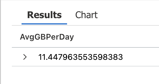
👉 Let’s break down the first iteration of this query and then discuss how we can clean it up and make it more efficient. This started out as a quick and dirty way to grab your daily average ingest, but as we’re about to learn, there’s more than one way to peel this KQL potato!
1.	search *                     //<-- Query Everything

2.	| where TimeGenerated > (30d)          //<-- Check the past 30 days

3.	| where _IsBillable == true  //<-- Only include billable ingest volume

4.	| summarize TotalGB = round(sum(_BilledSize/1000/1000/1000)) by bin(TimeGenerated, 1d)       //<-- Summarize billable volume in GB using the _BilledSize table column

5.	| summarize avg(TotalGB)     //<-- Summarize and return the daily average
Continuous Improvement:
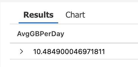
The most blatant offense here, is that I’m burning resources crawling through everything using “search *” in line 1 instead of specifying a table. This means that this query can take forever and even time-out in larger environments (after about 10 minutes). In the next iteration of this query, we query the Usage table instead to achieve the same results in less time. Try it out yourself in the free demonstration workspace and see the difference:
1.	Usage   //<-- Query the USAGE table (instead of "search *" to query everything)

2.	| where TimeGenerated > (30d)          //<-- Check the past 30 days

3.	| where IsBillable == true            //<-- Only include billable ingest volume

4.	| summarize GB= sum(Quantity)/1000 by bin(TimeGenerated,1d) //<-- Summarize in GBs by Day

5.	| summarize AvgGBPerDay=avg(GB)       //<-- Take the average
Continuous Improvement – Now What? Calculate Cost, of Course!
Now we have an efficient query to return the daily average ingest, but why stop there? The next question I’m almost always immediately asked next is “but what does that cost?” 🤑
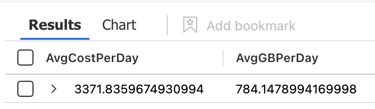
💡This next iteration includes an attempt to calculate average cost, and does so by introducing a rate variable (this variable holds your effective cost per GB based on your commitment tier. To find your effective cost per GB, check out my previous cost optimization blog post where this is covered in greater detail) and leveraging the percentiles function.
1.	let rate = 4.30;         //<-- Effective $ per GB rate for East US

2.	Usage	//<-- Query the USAGE table (instead of "search *" to query everything)

3.	| where TimeGenerated > ago(30d)          //<-- Check the past 30 days

4.	|where IsBillable == true 		//<-- Only include billable ingest volume

5.	|summarize GB= sum(Quantity)/1000 by bin(TimeGenerated,1d) //<-- Summarize GB/Day

6.	|extend Cost=GB*rate	//<-- calculate average cost

7.  | summarize AvgCostPerDay=percentiles(Cost,50),AvgGBPerDay=percentiles(GB,50) //<-- Return the 50th percentile for Cost/Day and GB/Day
Continuous Improvement - Underlying Query Logic and Presentation…
My grievances against the above query are as follows: Leveraging the percentiles function to take the 50th percentile is not technically the true average, but the closest actual cost to the median. Depending on the size of your environment, this can amount to a significant deviation from the true average. Last but not least, the output is just ugly too. Let’s fix that in our next query! 👇
1.	let rate = 4.30;         //<-- Effective $ per GB rate for East US

2.	Usage   //<-- Query the USAGE table (instead of "search *" to query everything)

3.	| where TimeGenerated > ago(30d)     //<-- Check the past 30 days

4.	| where IsBillable == true           //<-- Only include billable ingest volume

5.	| summarize GB= sum(Quantity)/1000 by bin(TimeGenerated,1d)     //<-- break it up into GB/Day

6.	| summarize AvgGBPerDay=avg(GB)      //<-- take the Average

7.	| extend Cost=AvgGBPerDay * rate     //<-- calculate average cost

8.	| project AvgGBPerDay=strcat(round(AvgGBPerDay,2), ' GB/Day'), AvgCostPerDay=strcat('$', round(Cost,2), ' /Day')    //<-- This line is tricky. I convert everything to string in order to prepend '$' and append ' /Day' to make the results more presentable
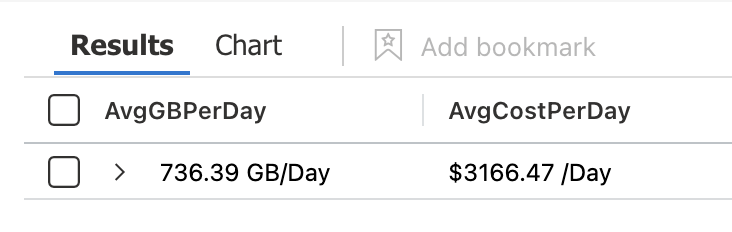
Much Better👆
In this post, we accomplished the following:
- ✓ Craft basic a basic, quick n’ dirty query that gets the job done
- ✓ Improve the efficiency and thus the time it takes to return results
- ✓ Improve upon the underlying query logic for more meaningful results
- ✓ Improve the end result presentation
- ✓ Understand the different layers of complexity for future query improvements
- ✓ Build something awesome 😎
📚 Want to go deeper?
My Toolbox books turn real Microsoft security telemetry into defensible operations:

🧰 PowerShell Toolbox Hands-On Automation for Auditing and Defense

🛠️ KQL Toolbox: Turning Logs into Decisions in Microsoft Sentinel

📖 Ultimate Microsoft XDR for Full Spectrum Cyber Defense
Real-world detections, Sentinel, Defender XDR, and Entra ID — end to end.
👆 Everything you’ve seen here — and much more — is in here 👆
⚡Thanks to everyone who’s already picked up a copy — your support means a lot. If you’ve read it and found value, please consider leaving a quick rating or review on Amazon. It genuinely helps the book reach more defenders.